While SCPT has been applied around the world for decades, recent years have seen a dramatic increase in the use of this soil investigation technique. Whether to provide input for the design of monopiles for offshore wind farms or the tracks for high-speed trains, or to assess the potential impact of seismic activity in areas where that kind of activity is a relatively new phenomenon.
As such, there is considerable interest in geotechnical in-situ soil investigation methods that provide accurate estimates of the shear and compression wave velocities (VS and VP respectively) in the soil. These parameters form the core of mathematical theorems to describe the soil’s elasticity/plasticity and are used to predict the responses including; settlement, liquefaction and failure to imposed loads such as from foundations, rotating equipment, earthquakes, trains travelling at high speeds or explosions.
You can read the full article below or download it as PDF.
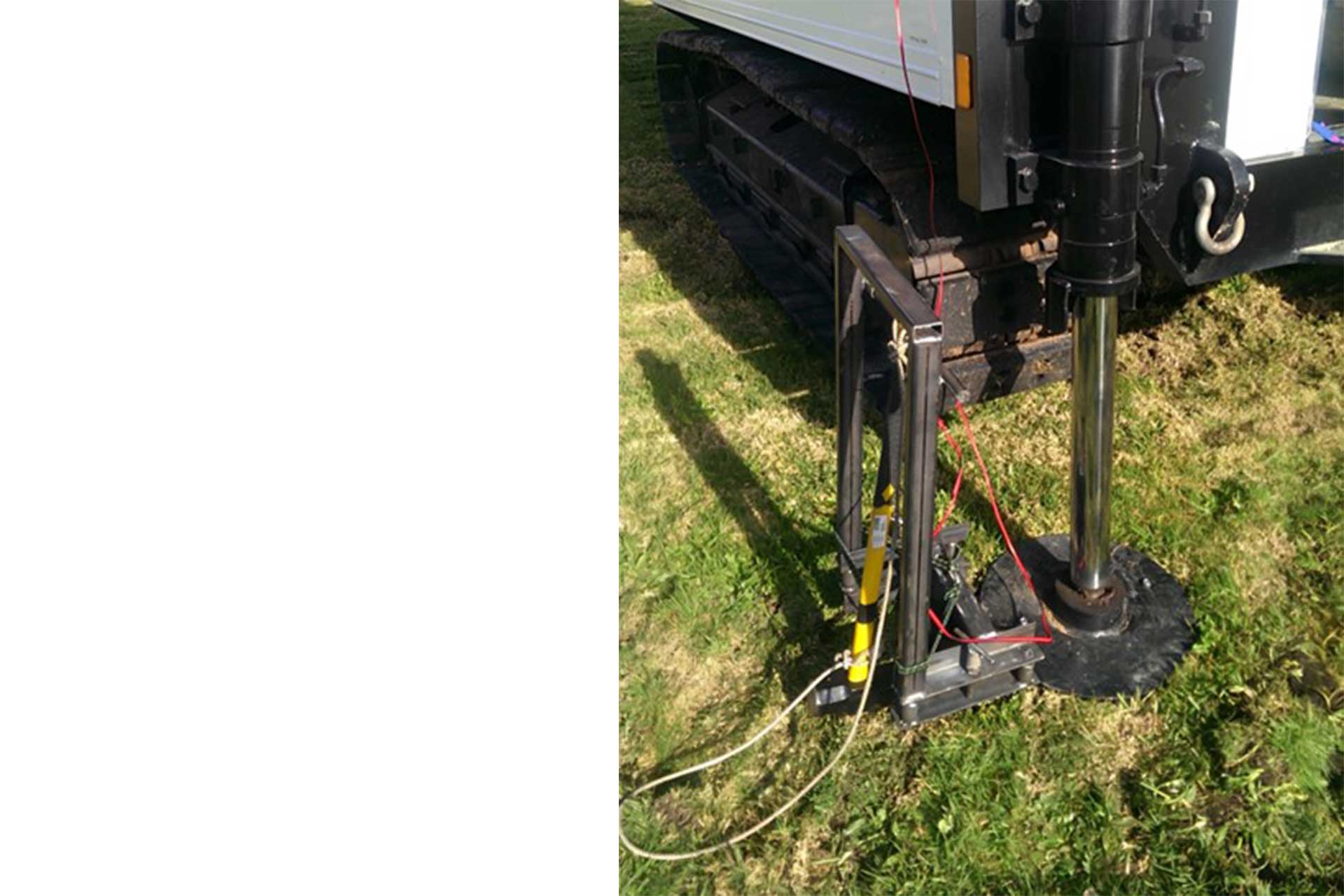
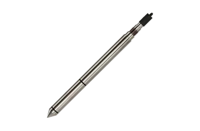
One of these soil investigation methods is Seismic Cone Penetration Testing (SCPT), whereby a seismic module is mounted behind the cone during a regular cone penetration test. At predefined depths the cone penetration test is paused, at which time a seismic source is used to generate a seismic wave at the ground surface. When the SCPT objective is to determine the shear wave velocity, this source can be as simple as a plate that is pushed into the ground, e.g. using the outrigger of CPT rig, and then hit by a hammer, shown in Figure 1 above.
The seismic module contains one or multiple seismic sensors, either geophone(s) or accelerometer(s), that are used to register the arrival of the seismic wave. As the hammer hits the plate the data recording system is triggered to begin recording the response of the seismic sensor(s). This process is repeated at all predetermined depths, which then generates a profile similar to that shown in Figure 2 below.
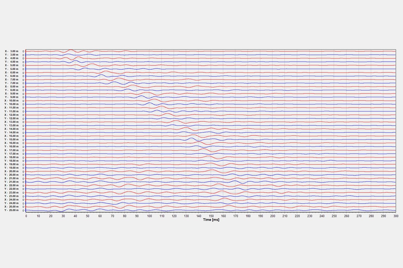
Here a biaxial sensor, reading the sensor response in the X and Y direction, was used between a depth of 3 and 25 metres, at 1 metre intervals, to determine the shear wave velocity profile.
From these results the time the shear wave requires to travel from the source to the sensor is then determined for each test depth, which is then used to calculate the shear wave velocity profile as a function of depth.
While the test is relatively easy to perform, in order to obtain reliable results there are some aspects that require the proper attention.
And finally, an appropriate analysis method must be used to first isolate the seismic wave signature from the recorded responses and then convert the arrival times to interval velocities.
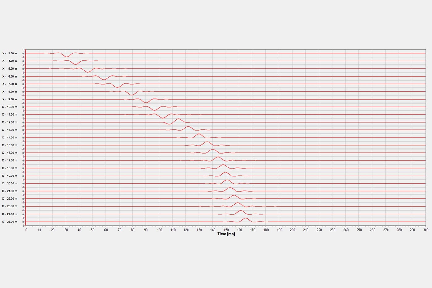
Figure 3 above is the plot with the sensor responses shown above after feature isolation was applied. While the conversion of arrival times to interval velocities seems as obvious as simply dividing the difference in the straight line distance between source and the sensor at two depths by the difference in the time required by the seismic wave to travel to those depths, the reality is much more complex.
The seismic wave does not travel in a straight line though the soil. Instead, the wave travels along a path that takes the least amount of time to go from the source to the sensor. Even though this fact, the so-called Fermat’s Principle or the Principle of the Least Time, has been known for centuries (it was first formulated by Pierre de Fermat in 1662), it is still widely ignored when SCPT data are analysed.
In addition, the analysis method must take into account source wave refraction that occurs when the source wave travels through the interface between soil layers. This principle is defined by Snell’s Law, which was formulated some 400 years ago, and illustrated in Figure 4 below.

This schematic illustrates the radial offset of the seismic source (X), the various depths of the seismic sensor (Z) and the travel path of the seismic wave through the various layers(d).
SCPT is specified and performed more widely and more frequently. This means that companies will have to become familiar with this technique, and Royal Eijkelkamp is ideally suitable to partner in that effort. The data acquisition hardware and software are part of the CPT product range and moreover, our specialists would be happy to assist in gaining a better understanding of this soil investigation technique, both when it comes to data acquisition and data analysis.
For more information about these products please visit our CPT product category, or feel free to contact our CPT specialists via CPT@eijkelkamp.com.